1 · Overview
What we set out to show
Problem
Weather, soil and crop records for Philippine provinces sit with different agencies in different formats, so they are rarely read together. We merged them into one dataset and charted it to see how growing conditions differ between provinces, how they changed over ten years, and how they line up with palay and corn yield.
Research questions
- How do seasonal rainfall, temperature and evapotranspiration relate to palay and corn yield?
- What trends show in rainfall, temperature and yield from 2015 to 2024, especially in El Niño years?
- Which weather, soil and yield variables move together?
- Which provinces group together on standardized climate, soil and yield?
- How do the ggplot2 and Seaborn versions compare?
2 · Dataset
Three public sources, one row per province and year
- 16provinces (top palay + corn producers)
- 10years, 2015–2024
- 58,448daily weather records
- 320province-crop-year yield rows
| Source | Variables | Rows × columns | Coverage |
|---|---|---|---|
| Open-Meteo Historical Weather API | Mean, max and min temperature, rainfall, FAO reference evapotranspiration, solar radiation, relative humidity, soil moisture 0–7 cm (all numeric) | 58,448 × 10 | Daily, 2015–2024, one point per province |
| ISRIC SoilGrids 2.0 | pH, clay, sand, silt, organic carbon, nitrogen, CEC, bulk density at 0–5, 5–15 and 15–30 cm (numeric) | 384 × 6 | Static, one point per province |
| PSA OpenSTAT, tables 0012E4EVCP0 and 0022E4EAHC0 | Palay and corn production (t) and area harvested (ha) (numeric); province and crop (text) | 4,360 × 5 | Annual, all provinces, 2015–2024 |
The merged file crop_panel.csv has 320 rows × 25 columns: province, region, island group, crop and year, plus area, production, yield, 8 weather and 8 soil columns.
3 · Preparation
What we did to the data
Acquisition
A Python script queried each API once and saved the replies as CSV, so every chart is reproducible without calling an API again. Each province is represented by one hand-picked point in its main cropland. Two points (Isabela, Sultan Kudarat) were moved after SoilGrids returned no data at the first spot.
Missing values and duplicates
Weather: 0 missing, 0 duplicate days. Soil: 0 missing after the two moves. Yield: 0 missing for the 16 provinces.
Outliers
Yields outside 1.5 × IQR per crop were flagged, not removed. The five flagged rows are all Nueva Ecija palay from 2020 to 2024 (5.9–6.3 t/ha), a real result of the country's most irrigated rice province.
Transformation
- PSA's 2022 split of Maguindanao into del Norte and del Sur was summed back into one province. Negros Occidental's 2024 row under the new Negros Island Region was joined to its earlier series.
- SoilGrids integers converted to units (pH ÷ 10, g/kg ÷ 10 and so on), then combined into a 0–30 cm mean weighted by layer thickness.
- Daily weather summed or averaged to months and years. Wet-season rainfall is June to November.
- Yield = production ÷ area harvested, in t/ha.
Standardization
For the cluster maps each variable was converted to a z-score (mean 0, SD 1) across the 16 province averages, so millimetres of rain and pH units weigh the same.
4 · Exploratory data analysis
Descriptive statistics
| Variable | Unit | Mean | SD | Min | Median | Max |
|---|---|---|---|---|---|---|
| Annual rainfall | mm | 2,875 | 883 | 1,382 | 2,714 | 5,773 |
| Wet-season rainfall | mm | 1,858 | 488 | 1,021 | 1,798 | 3,331 |
| Mean temperature | °C | 26.20 | 1.31 | 22.24 | 26.46 | 28.01 |
| Mean daily maximum | °C | 30.27 | 1.77 | 25.17 | 30.52 | 33.05 |
| Reference evapotranspiration | mm/yr | 1,420 | 124 | 1,104 | 1,414 | 1,728 |
| Solar radiation | MJ/m²/day | 18.17 | 0.86 | 15.94 | 18.22 | 20.10 |
| Relative humidity | % | 82.07 | 3.85 | 73.99 | 82.71 | 89.42 |
| Soil moisture, 0–7 cm | m³/m³ | 0.35 | 0.05 | 0.26 | 0.35 | 0.47 |
| Palay yield | t/ha | 4.09 | 0.75 | 2.47 | 4.05 | 6.28 |
| Corn yield | t/ha | 3.92 | 1.44 | 1.32 | 3.96 | 7.00 |
| Soil pH (water) | pH | 5.75 | 0.47 | 5.05 | 5.61 | 6.53 |
| Clay, 0–30 cm | % | 38.64 | 5.42 | 25.12 | 40.07 | 50.65 |
| Organic carbon, 0–30 cm | g/kg | 31.61 | 23.07 | 12.97 | 21.96 | 104.68 |
| CEC, 0–30 cm | cmol(c)/kg | 21.24 | 6.77 | 11.65 | 19.48 | 34.62 |
Initial observations
- Rainfall varies far more than temperature. Annual totals run from 1,382 mm to 5,773 mm (Lanao del Sur averages 4,669 mm), while mean temperature stays within about 6 °C. Rain peaks in July (365 mm on average) and bottoms out in February (102 mm).
- Corn yield spreads twice as wide as palay yield (SD 1.44 vs 0.75 t/ha), from 1.36 t/ha in Leyte to 6.72 t/ha in Tarlac.
- 2015 was the driest year in the set (2,118 mm average) and 2022 the wettest (3,677 mm).
- Maguindanao's organic carbon (104.7 g/kg) is three times the next province. Its point lies by the Liguasan Marsh; the value is kept.
5 · Scatterplot
Wet-season rainfall barely moves yield
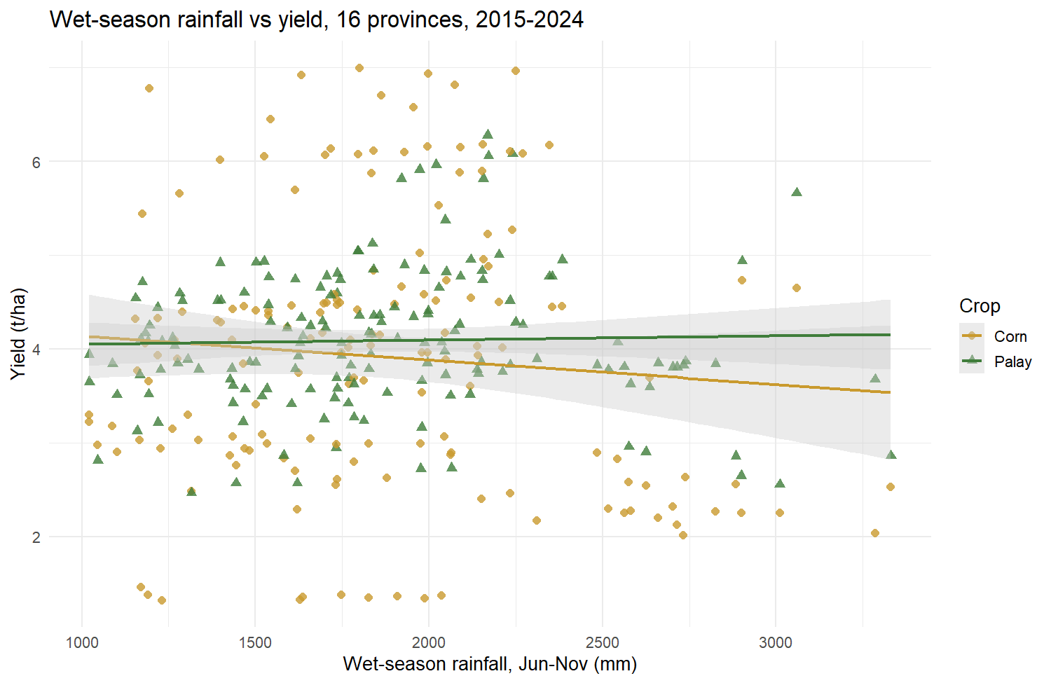
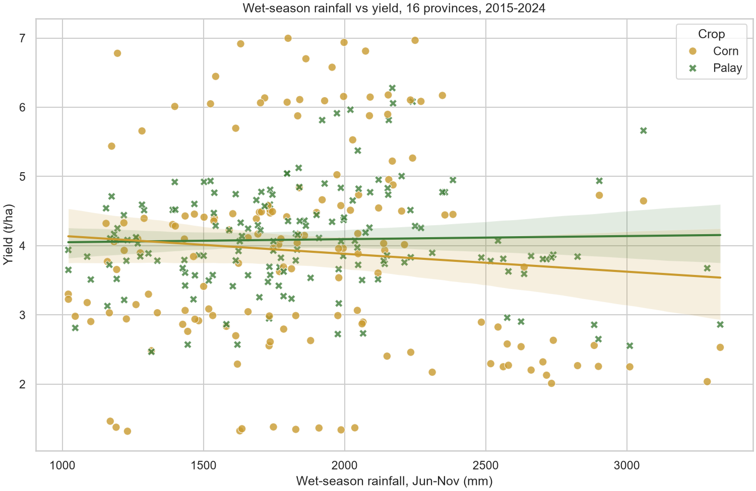
Variables: wet-season rainfall, June–November (x) against yield in t/ha (y), one point per province, crop and year (n = 320), with a linear fit and 95% band per crop.
Not rendered yet. Run Rscript r/charts.R.
Not rendered yet. Run python python/charts.py.
Interpretation
Neither crop has a meaningful linear link to wet-season rainfall. For palay r = 0.03 (p = 0.71); for corn r = −0.09 (p = 0.27), about 0.26 t/ha less per extra 1,000 mm. The vertical spread at any rainfall level is much larger than the trend, which points to differences between provinces (irrigation, soil, variety) rather than rain itself. The wettest points, above 2,400 mm, come from six provinces including Lanao del Sur and Negros Occidental, which also have low corn yields.
Comparison
Both show the same points and fits. ggplot2 maps colour and shape in one aes() call and draws the fits with one geom_smooth(). Seaborn needs a separate regplot() per crop to colour each fit, but its bands take the crop colour by default, which makes them easier to tell apart than ggplot2's grey ones.
6 · Line plot
Yields rose over the decade and dipped in El Niño years
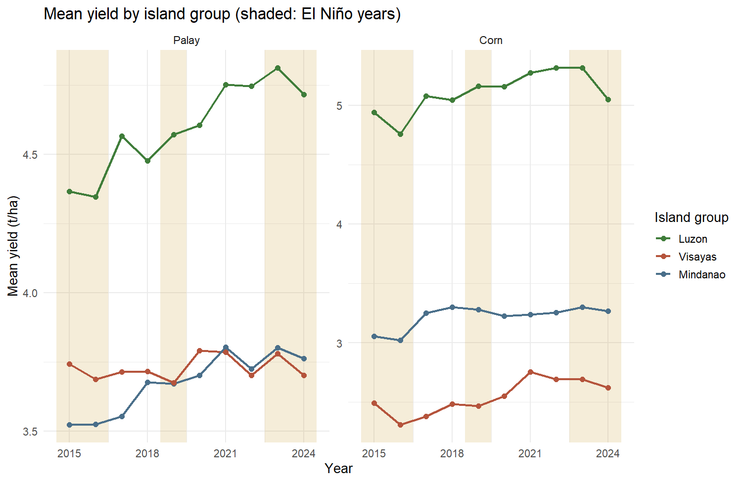
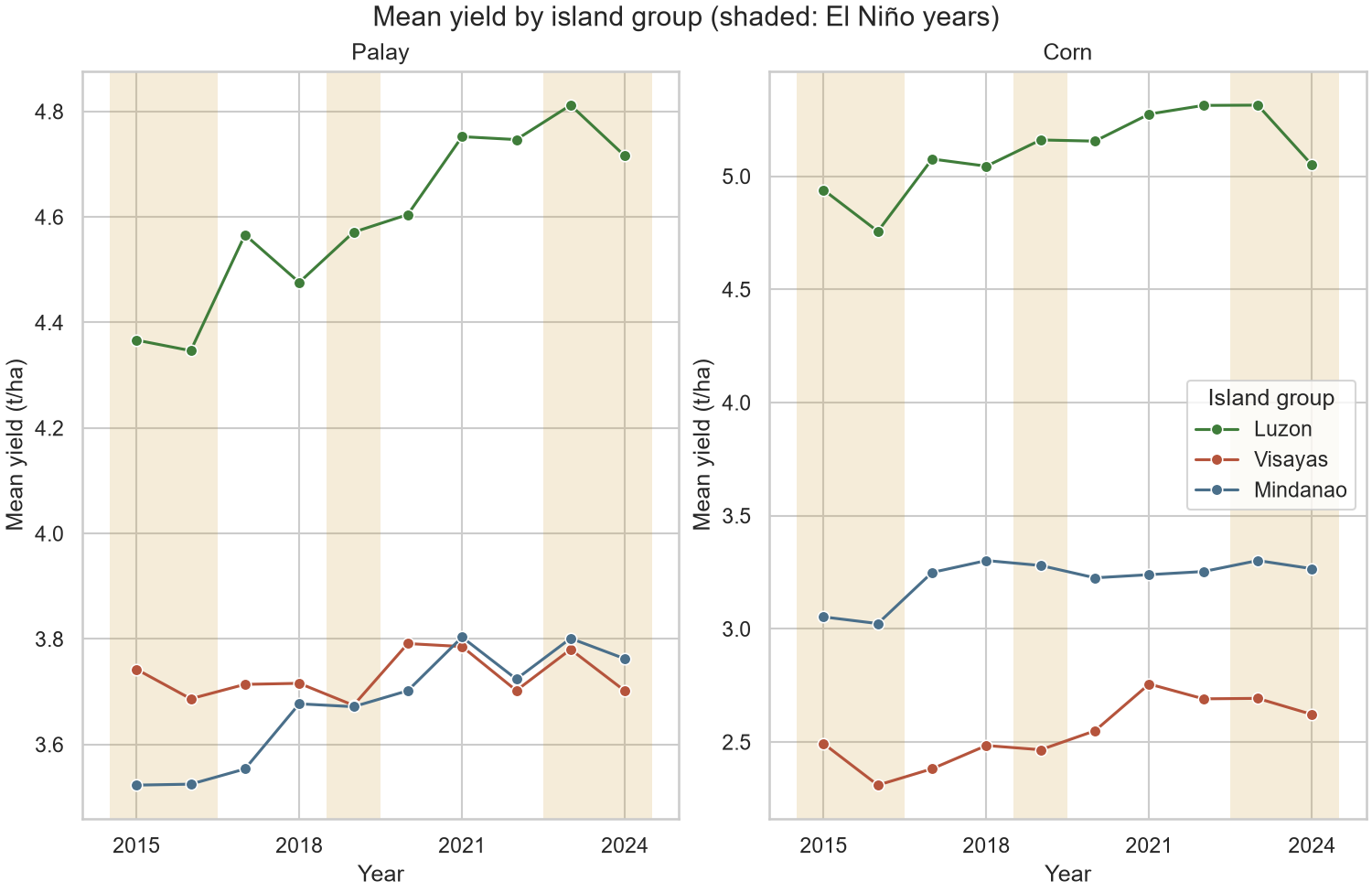
Variables: year (x) against mean yield in t/ha (y) for each island group, faceted by crop. Shaded bands mark the El Niño years 2015–16, 2019 and 2023–24.
Not rendered yet. Run Rscript r/charts.R.
Not rendered yet. Run python python/charts.py.
Trend analysis
Across the 16 provinces, mean palay yield rose from 3.93 t/ha in 2015 to 4.17 in 2024 and corn from 3.77 to 3.93. Luzon stays on top every year (palay 4.6, corn 5.1 t/ha on average); Visayas corn is lowest (2.5 t/ha). Luzon palay gained the most (4.37 to 4.72 t/ha); Visayas palay stayed flat near 3.7.
El Niño years. 2016 was the low point for Luzon (palay 4.35, corn 4.76 t/ha) and Visayas corn (2.31 t/ha). Luzon corn also fell from 5.31 in 2023 to 5.05 t/ha in 2024. The 2019 event left no clear mark. These dips line up with the drought years but do not prove the drought caused them.
Comparison
ggplot2 needs the means computed first (aggregate()) and the El Niño bands as a data frame for geom_rect(); facet_wrap() then splits the crops in one line. Seaborn averages inside lineplot(), but the facets and bands need a matplotlib loop with axvspan().
7 · Heatmap
Soil chemistry tracks yield more closely than rainfall does
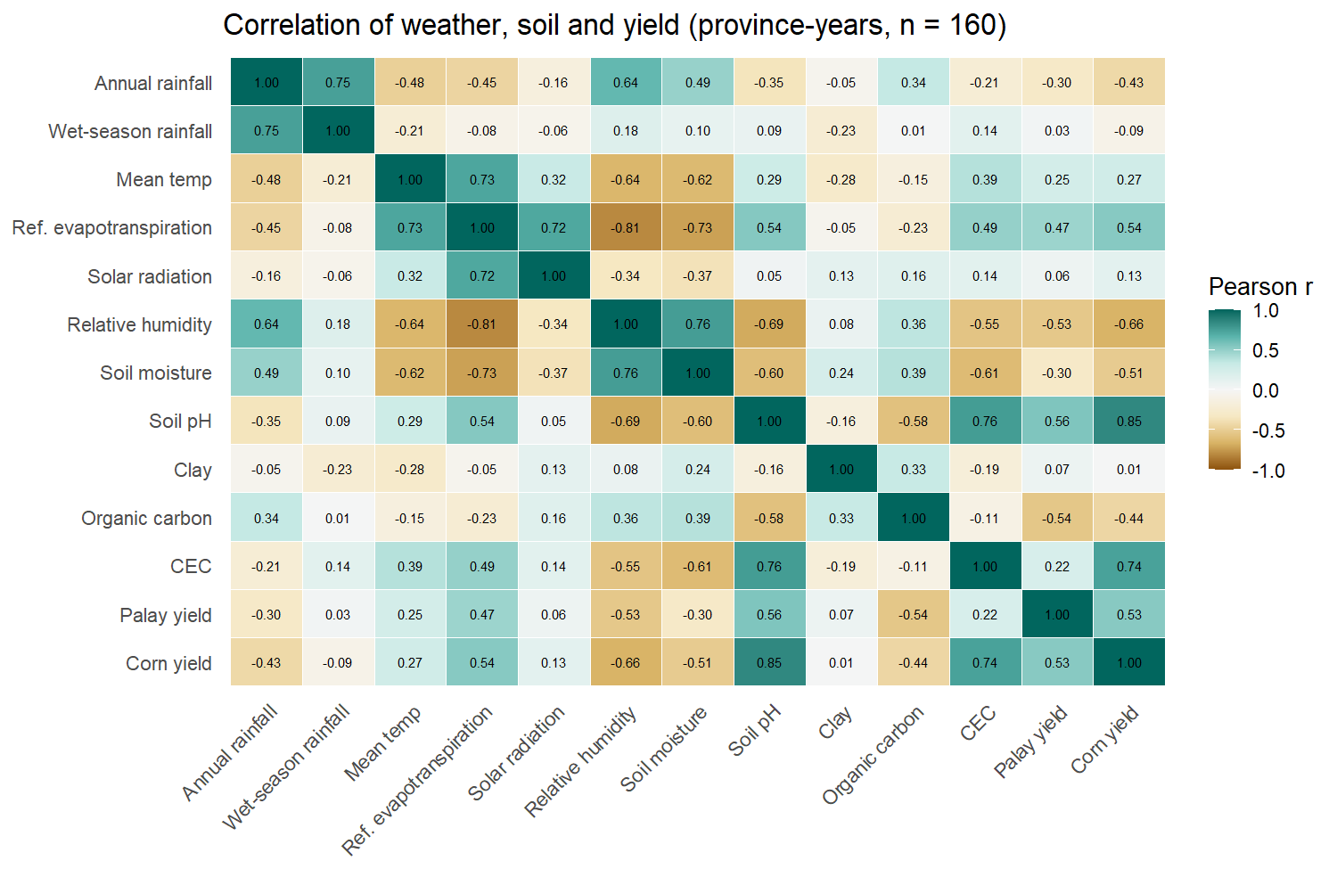
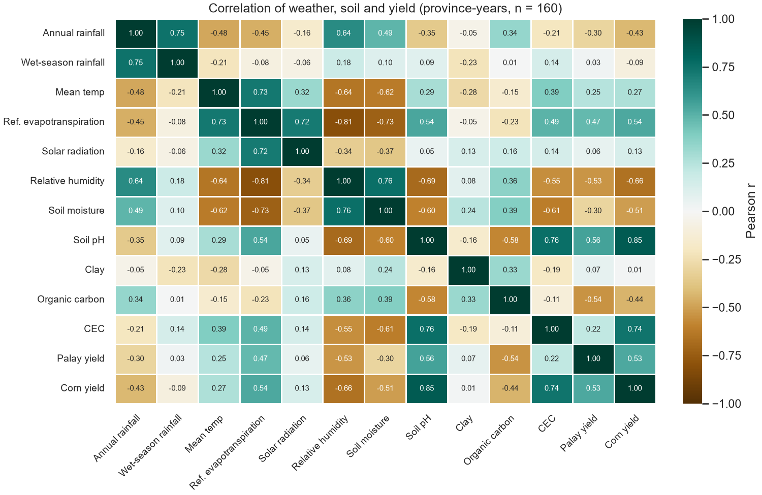
Variables: Pearson correlation between 13 weather, soil and yield variables over the 160 province-years.
Not rendered yet. Run Rscript r/charts.R.
Not rendered yet. Run python python/charts.py.
Colour scale
A diverging brown-to-teal scale (ColorBrewer BrBG) fixed at −1 to 1: teal cells move together, brown cells move in opposite directions, and near-white cells are unrelated. The diverging scale keeps zero in the middle, so sign is readable at a glance.
Interpretation
- Corn yield follows soil pH (r = 0.85) and CEC (0.74) closely. Palay yield follows pH too (0.56) but more weakly.
- Both yields fall with relative humidity (palay −0.53, corn −0.66) and rise with evapotranspiration (0.47, 0.54). The drier, sunnier plains of Central Luzon drive this.
- Rainfall is weak against yield (annual −0.30 and −0.43, wet-season near 0), matching the scatterplot.
- Soil values are fixed per province, so their correlations compare provinces, not years.
Comparison
The numbers match exactly. Seaborn draws the annotated heatmap in one call from the correlation matrix. ggplot2 has no heatmap function, so the matrix is reshaped to long form and drawn with geom_tile() plus geom_text(), which is more code but gives full control over each layer.
8 · Cluster map
Central Luzon stands apart; the rest split into upland and lowland groups
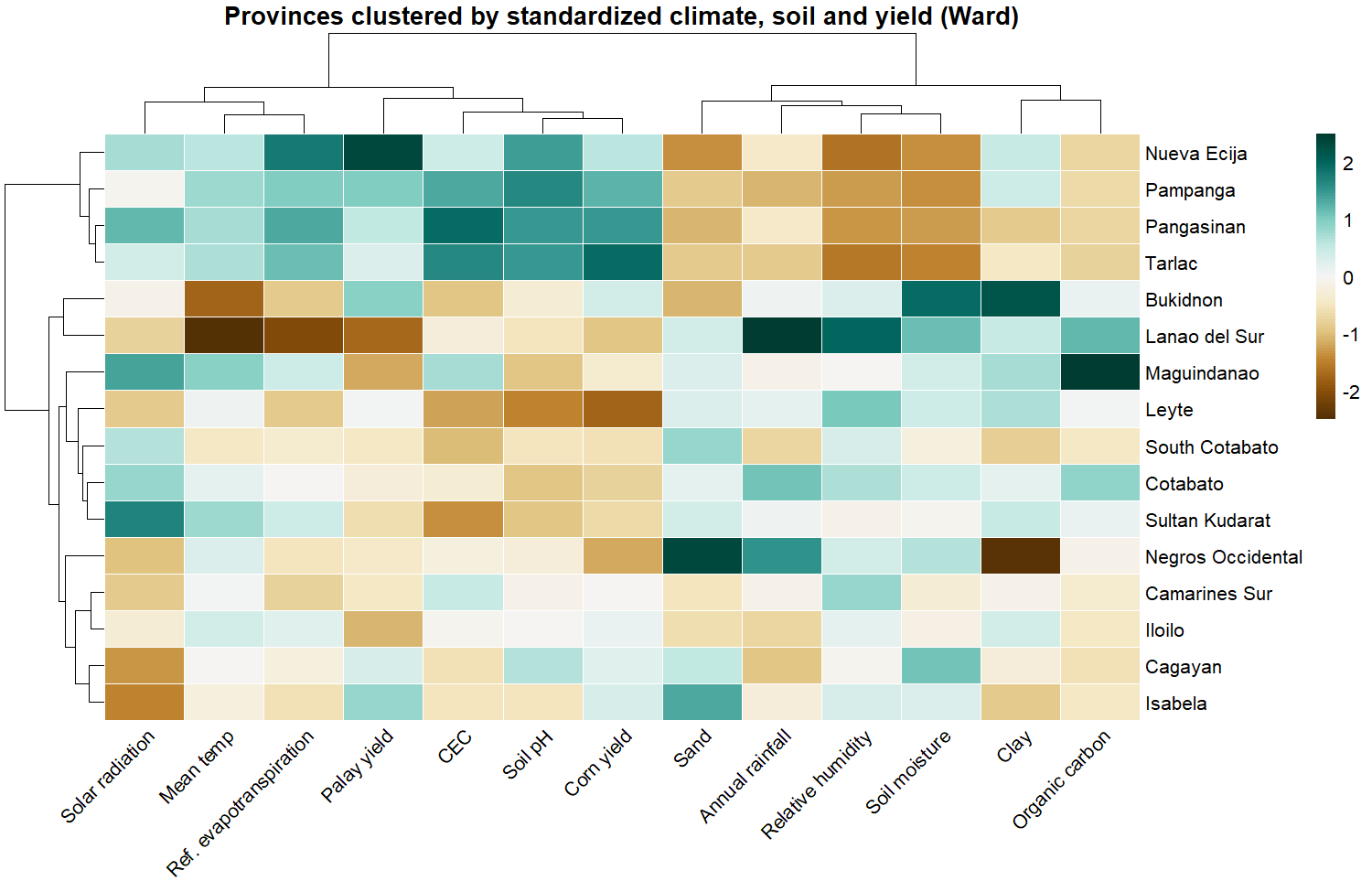
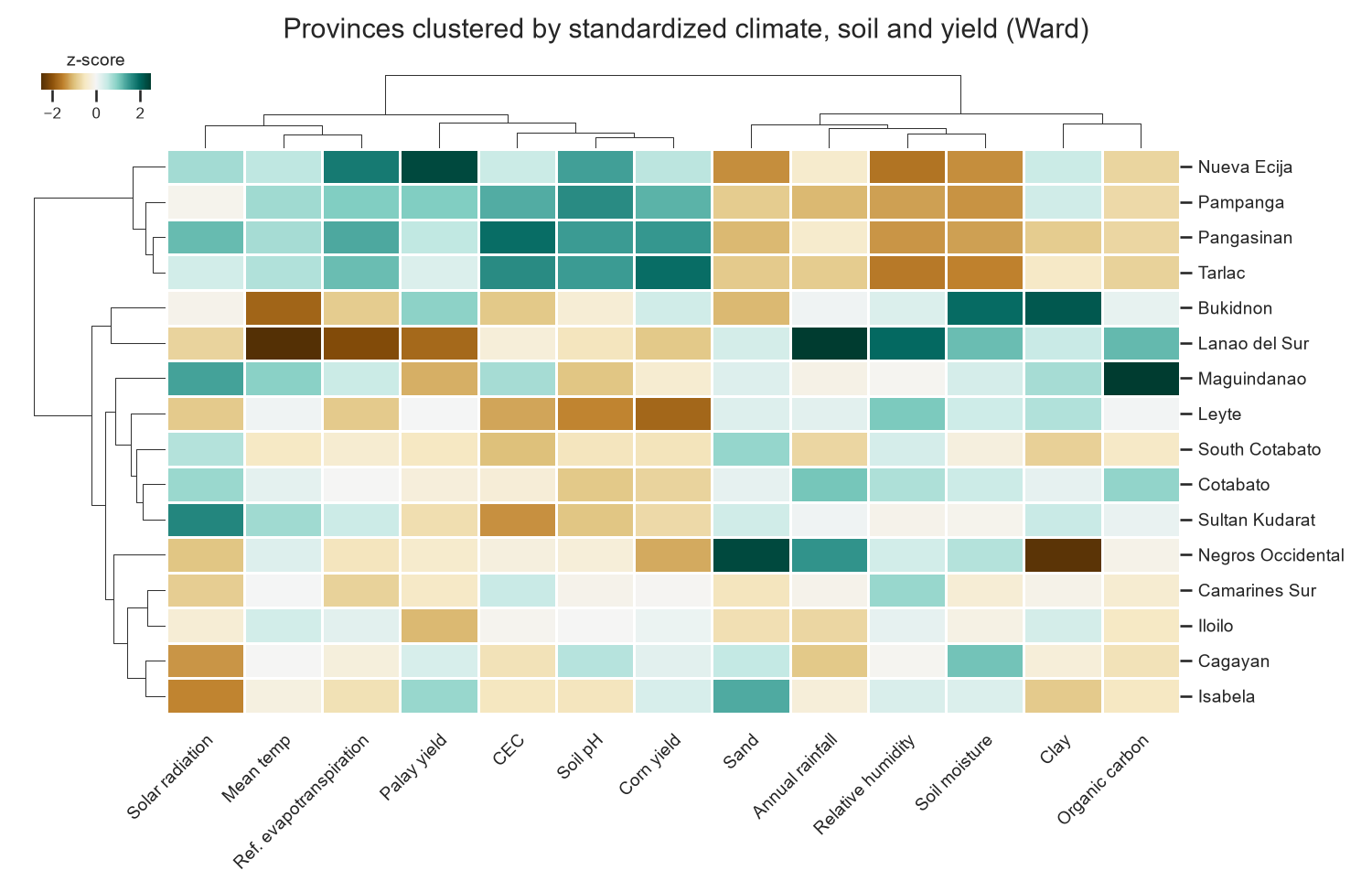
Variables: 13 province averages (climate, soil, palay and corn yield), each z-scored. Method: hierarchical clustering, Euclidean distance, Ward linkage, on rows and columns.
Not rendered yet. Run Rscript r/charts.R.
Not rendered yet. Run python python/charts.py.
Groups (cut at four clusters)
| Group | Provinces | What sets it apart |
|---|---|---|
| Central Luzon plain | Nueva Ecija, Pampanga, Pangasinan, Tarlac | Highest yields, highest pH and CEC, low humidity and soil moisture |
| Cool uplands | Bukidnon, Lanao del Sur | Lowest temperature and evapotranspiration; Lanao del Sur has the most rain |
| Mindanao lowlands + Leyte | Maguindanao, Cotabato, South Cotabato, Sultan Kudarat, Leyte | Low soil pH (5.05–5.50) and below-average corn yield |
| Mixed lowlands | Isabela, Cagayan, Iloilo, Camarines Sur, Negros Occidental | Near-average on most variables; Negros Occidental is sandy and wet |
The groups follow landform more than island group: Mindanao provinces fall into two different clusters, and Visayas provinces into two. On the column side, yield, pH, CEC and evapotranspiration cluster together against humidity, soil moisture and rainfall, the same split the heatmap shows.
Comparison
Both tools produced the same tree, since pheatmap's ward.D2 and SciPy's ward are the same method. pheatmap draws the whole figure in one call but is a separate package outside ggplot2. Seaborn's clustermap() is built in, but placing the colour bar and fitting long labels took manual layout code.
9 · Comparative analysis
ggplot2 and Seaborn side by side
| Aspect | ggplot2 (R) | Seaborn (Python) |
|---|---|---|
| Code structure | Layers added with +; one grammar for all four charts except the cluster map (pheatmap) | One function per chart type; matplotlib needed for bands, facets and layout |
| Data shape | Prefers long data; the correlation matrix had to be reshaped | Takes wide matrices directly for heatmap and clustermap |
| Defaults | Clean minimal theme; grey confidence bands; legend outside the plot | Grid theme; bands in the series colour; legend inside the plot |
| Customization | Facets, scales and labels in one chain | Fine control through matplotlib, at the cost of more lines |
| Lines of chart code | 72, including the pheatmap call | 94, including layout fixes for the cluster map |
| Best fit here | Faceted trend charts and layered annotations | Correlation heatmaps and cluster maps in one call |
Both read the same CSVs and produce the same numbers, so the choice comes down to workflow. R needed fewer lines overall. R was quicker for the line plot, Python for the heatmap.
10 · Preliminary findings
What the charts show so far
- Rain alone does not explain yield. Wet-season rainfall has no significant linear link to palay (r = 0.03) or corn yield (r = −0.09). (Scatterplot)
- Yields rose over the decade. Mean palay yield went from 3.93 to 4.17 t/ha and corn from 3.77 to 3.93 t/ha between 2015 and 2024. (Line plot)
- El Niño years coincide with dips. 2016 was the lowest year for Luzon palay and corn and for Visayas corn, and Luzon corn fell again in 2024. (Line plot)
- Soil and dryness go with high yield. Corn yield correlates with soil pH (0.85) and CEC (0.74) and negatively with humidity (−0.66). (Heatmap)
- Provinces group by landform. The four Central Luzon plain provinces form their own cluster with the highest yields; Bukidnon and Lanao del Sur form a cool upland pair. (Cluster map)
Associations here are descriptive. Province-level soil and one weather point per province cannot separate the effect of irrigation, variety or farm practice.